Performing Analyses
Examining a Simple Workflow
Let’s first create a concentration-time plot of the Theophylline data set:
library(reportifyr)library(ggplot2)library(dplyr)
data <- Theoph
p <- ggplot(data, aes(x = Time, y = conc, group = Subject)) +  geom_point() +  geom_line() +  theme_bw() +  labs(x = "Time (hr)", y = "Theophylline concentration (mg/L)")
p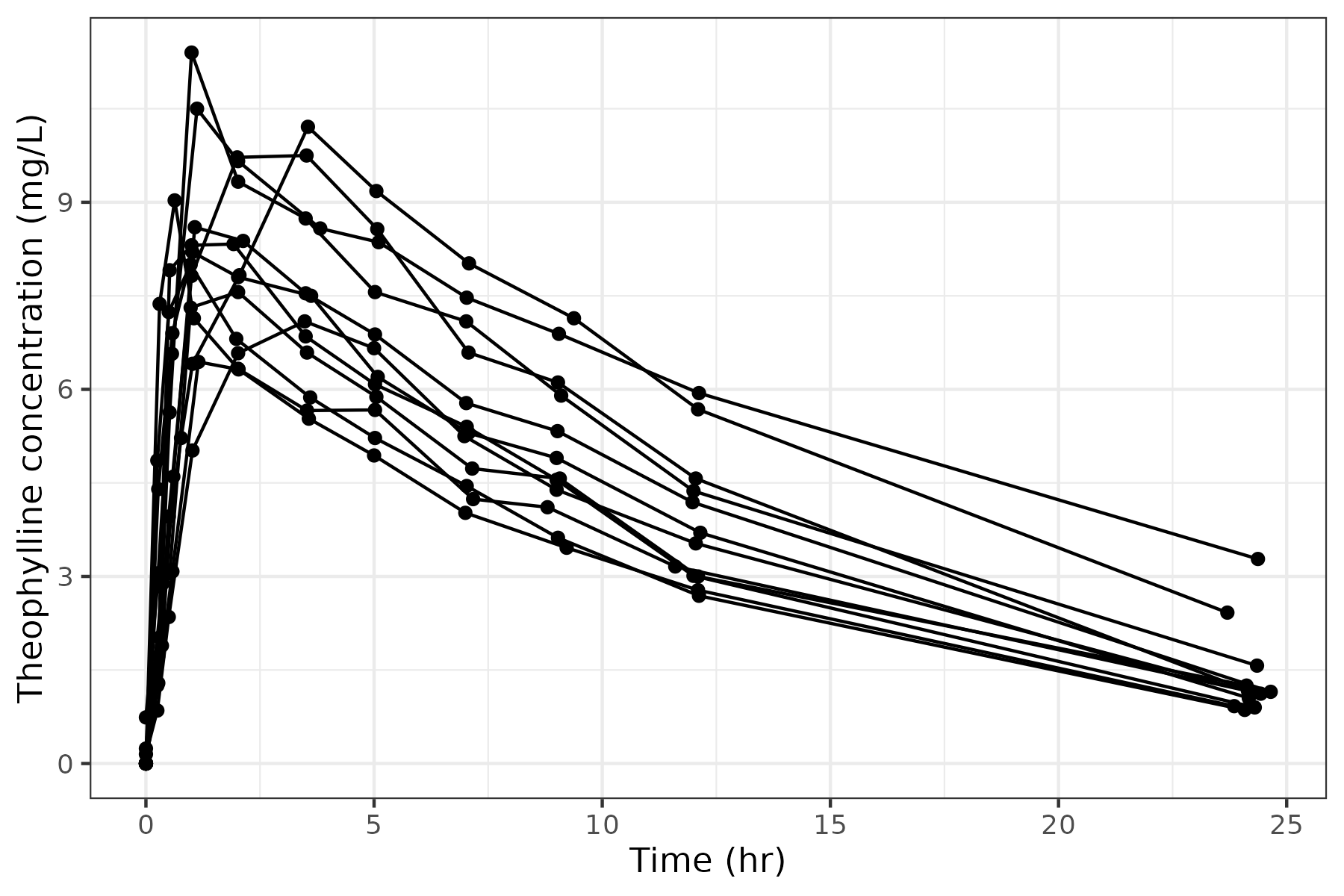
Saving the Figure and Creating Metadata
If we want to include this plot into the report we’ll need to save this
figure to the OUTPUTS/figures subdirectory. There are two separate
processes to accomplish this - the easiest way is to call the wrapper
function ggsave_with_metadata():
figures_path <- here::here("OUTPUTS", "figures")plot_file_name <- "theoph-pk-plot.png"
ggsave_with_metadata(  filename = file.path(figures_path, plot_file_name),  plot = p,  width = 6,  height = 4)
Alternatively you could call ggplot2::ggsave() and then call
write_object_metadata():
ggplot2::ggsave(  filename = file.path(figures_path, plot_file_name),  plot = p,  width = 6,  height = 4)
write_object_metadata(object_file = file.path(figures_path, plot_file_name))
Both processes give the same final result, however, severing the tie between saving a figure/table (artifact) and writing its metadata may lead to the these artifacts becoming out of sync.
Using Metadata to Standardize Footnotes
This brings us to metadata. reportifyr uses metadata to create a
record of the artifact being inserted into the Microsoft Word document (report) to
aid in reproducibility and traceability.
Specifically, reportifyr uses a meta_type parameter to inject a portion of
standardized footnotes into the report. We can use the function get_meta_type()
to see what artifact meta_type values are currently saved in the
standard_footnotes.yaml within the ‘report’ subdirectory upon initialization.
We just need to provide the path to the standard_footnotes.yaml that we want
to pull meta_type from.
Below are the basic meta_type included automatically
within reportifyr. If a new meta_type is required for your report, simply follow
the formatting style in the standard_footnotes.yaml file to expand the list.
meta_type <- get_meta_type(here::here("report", "standard_footnotes.yaml"))
names(meta_type)[1] "logistic_plot"          "boxplot"                "TTE_plot"               "correlation_plot"       "GOF_plot"               "ETA_histogram"          "VPC"                    "kaplan-meier-plot"      "conc-time-trajectories" "linear-regression-plot" "probit-regression-plot"[12] "univariate"             "final"                  "full"                   "alternative"            "univariate_TTE"         "final_TTE"              "full_TTE"               "alternative_TTE"        "ER_summary"             "covariate_descriptive"  "frequency"[23] "probit-regression-fit"  "linear-regression-fit"  "cox-regression-fit"
Now, let’s re-save the plot object with the conc-time-trajectories meta_type
provided:
plot_file_name_meta <- "theoph-pk-plot-meta.png"
ggsave_with_metadata(  filename = file.path(figures_path, plot_file_name_meta),  plot = p,  meta_type = meta_type$`conc-time-trajectories`,  width = 6,  height = 4)
Using meta_type$ also allows for tab-completion to help you select the correct
meta_type! Let’s use the preview_metadata_files() to see the
difference when using a meta_type:
metadata <- preview_metadata_files(file_dir = figures_path)
knitr::kable(metadata)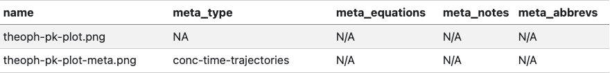
From the data frame, we can see that there are additional parameters that can be
saved as part of an artifact’s metadata using reportifyr’s wrapper functions
(i.e., meta_abbreviations, meta_equations, and meta_notes).
Similar to meta_type, we can retrieve a list of standardized meta_abbrevs
stored in the standard_footnotes.yaml by using get_meta_abbrevs():
meta_abbrevs <- get_meta_abbrevs(here::here("report", "standard_footnotes.yaml"))
names(meta_abbrevs)[1] "AUC"       "AGEBL"     "ALBBL"     "ALTBL"     "ASTBL"     "B2MBL"     "BSABL"     "BSTGBGE2"  "BSTGEQ3"   "CADC_21D"  "CADC_28D"  "CADC_42D"  "CADC_56D"  "CATABL"    "CAVGA_21D" "CAVGA_28D" "CAVGA_42D" "CAVGA_56D" "CAVGM_21D" "CAVGM_28D" "CMAXA"     "CMAXM"     "CNCEURO"   "CRPBL"[25] "CYTORSK"   "ECOGBEQ2"  "ECOGBGE1"  "GLAUCBL"   "HEPFCH"    "HISTDIAB"  "HSDRYEYE"  "HSIOSURG"  "IBMIBL"    "IGGBL"     "IGGFLG"    "KERABL"    "LDHBL"     "LENSTABL"  "MEDFL"     "MMIGTY"    "MMLCTY"    "MMTY"      "MPROTBL"   "PCD38"     "PRXGT3"    "PRXGT4"    "RACEBFLG"  "RACEWFLG"[49] "RENALFCH"  "SBCMABL"   "SCH"       "SCHCH"     "SEXN"      "SPLITB"    "STAGEBL"   "STRETCHB"  "TBILBL"    "WTBL"
Now, instead of saving the second figure (plot_file_name_meta) out again using
gg_save_with_metadata() and providing the additional arguments, let’s instead
use update_object_footnotes() to add a mock meta_abbrevs:
update_object_footnotes( file_path = file.path(figures_path, plot_file_name_meta), overwrite = TRUE, meta_abbrevs = c(meta_abbrevs$CMAXA))Once we have updated the footnotes for the second figure, let’s take one last preview of its metadata to confirm our changes.
metadata_file <- preview_metadata(file_name = file.path(figures_path, plot_file_name_meta))
knitr::kable(metadata_file)
Performing an Analyses
With a simple workflow examined, let’s perform an analysis computing
subject level pharmacokinetic parameters and then study level statistics of the
data set to generate an additional plot. We’ll compute maximum drug concentration
(CMAX), time to peak drug concentration (TMAX), and area under the
concentration-time curve (AUC) for the Theophylline data set before
performing a linear regression between baseline weight (WTBL) and AUC.
Generating a Figure for Use with reportifyr
calc_auc_linear_log <- function(time, conc) {  auc <- 0
  cmax_index <- which.max(conc)
  for (i in 1:(length(time) - 1)) {    delta_t <- time[i + 1] - time[i]
    if (i < cmax_index) {
      auc <- auc + delta_t * (conc[i + 1] + conc[i]) / 2    } else if (i >= cmax_index && conc[i + 1] > 0 && conc[i] > 0) {
      auc <- auc + delta_t * (conc[i] - conc[i + 1]) / log(conc[i] / conc[i + 1])    } else {
      auc <- auc + delta_t * (conc[i + 1] + conc[i]) / 2    }  }
  return(auc)}
pk_params <- data %>%  mutate(Subject = as.numeric(Subject)) %>%  group_by(Subject) %>%  summarise(    cmax = max(conc, na.rm = TRUE),    tmax = Time[which.max(conc)],    auc = calc_auc_linear_log(Time, conc),    wt = Wt %>% unique()  )
knitr::kable(pk_params)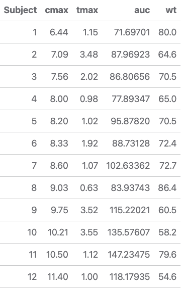
lr <- pk_params %>%  ggplot(aes(x = wt, y = auc)) +  geom_point() +  geom_smooth(method = "lm", formula = y ~ x, se = TRUE, color = "blue") +  theme_bw() +  labs(x = "Subject weight (kg)", y = "AUC (hr mg/L)")
lr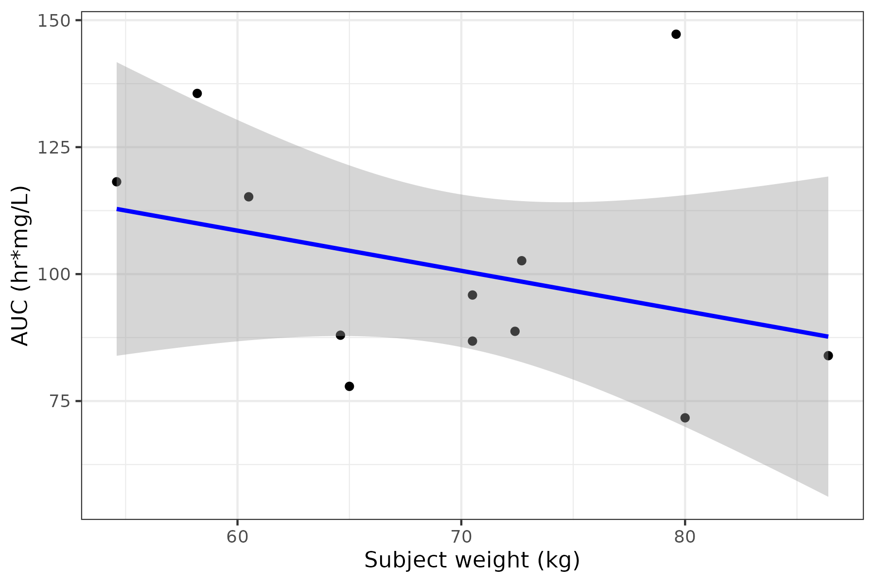
Let’s save this plot with the linear-regression-plot meta_type and the relevant
AUC meta_abbrevs.
plot_file_name <- "theoph-pk-exposure.png"
ggsave_with_metadata(  filename = file.path(figures_path, plot_file_name),  plot = lr,  meta_type = meta_type$`linear-regression-plot`,  meta_abbrevs = c(meta_abbrevs$AUC),  width = 6,  height = 4)
Generating a Table for Use with reportifyr
With our linear regression plot generated and saved, let’s now save out the pk_params
data frame to .csv using write_csv_with_metadata() so we can include it in
the report. We can pass in similar meta_type, meta_notes, and meta_abbrevs
arguments, if applicable, as well as any arguments that would be used in write.csv().
For this table, let’s use row.names = FALSE:
tables_path <- here::here("OUTPUTS", "tables")outfile_name <- "theoph-pk-parameters.csv"
write_csv_with_metadata(  object = pk_params,  file = file.path(tables_path, outfile_name),  meta_abbrevs = c(meta_abbrevs$AUC),  row.names = FALSE)
Similarly, let’s also save out the Theophylline data set to include in the
report. This time we will format the table using format_flextable() before saving
the table out as an .RDS file:
library(flextable)
data_outfile_name <- "theoph-pk-data.RDS"
table <- format_flextable(  data_in = data,  table1format = FALSE)
save_rds_with_metadata(  object = table,  file = file.path(tables_path, data_outfile_name))
At the end, we’ve generated two figures and two tables and saved them
alongside their metadata using reportifyr, allowing us to easily
incorporate them into our upcoming Drafting Reports!